Real-World Climate Analysis Case Study — dask_setup Recipe
This notebook walks through a complete scientific data processing workflow:
Generate a synthetic multi-year climate dataset
Quality-control the data (flag fill values, range checks)
Compute temporal aggregations — annual mean, seasonal climatology
Fit a linear temperature trend
Save processed outputs to Zarr
Generate summary plots (if matplotlib is available)
All steps are designed to work on a laptop using profile="development", and scale
to a full HPC node by switching to profile="climate_analysis".
Setup
import tempfile
import time
from pathlib import Path

import numpy as np
import pandas as pd
import xarray as xr

from dask_setup import setup_dask_client

try:
    import matplotlib.pyplot as plt
    PLOT = True
except ImportError:
    PLOT = False
    print("matplotlib not found — plots will be skipped")

try:
    import zarr
    ZARR = True
except ImportError:
    ZARR = False
    print("zarr not found — Zarr output will be skipped")

WORK_DIR = Path(tempfile.mkdtemp(prefix="climate_case_"))
print(f"Work dir: {WORK_DIR}")
print("Imports OK")
Work dir: /tmp/climate_case_k8aftkqg
Imports OK
1. Start Cluster
Use profile="development" for laptops. Switch to profile="climate_analysis" on a Gadi node.
client, cluster, tmp = setup_dask_client(
    profile="development",
    fallback_on_detection_failure=True,
)
print(f"Workers    : {len(client.nthreads())}")
print(f"Temp dir   : {tmp}")
if hasattr(cluster, 'dashboard_link'):
    print(f"Dashboard  : {cluster.dashboard_link}")
[setup_dask_client] Configuration summary
temp/spill dir: /tmp/dask-3153
Workers: 2 | threads/worker: 2 | processes: True
Memory: total ~15.6 GiB | usable ~7.6 GiB | per-worker ~3.8 GiB
Compression: spill=auto | comm=False
Workers    : 2
Temp dir   : /tmp/dask-3153
Dashboard  : http://127.0.0.1:38797/status
2. Generate Synthetic Climate Dataset
We create 10 years of daily data on a coarse global grid — temperature with a warming trend and a seasonal cycle, plus precipitation with log-normal noise.
YEARS = 10
N_TIME = 365 * YEARS
LAT = np.linspace(-90, 90, 36)
LON = np.linspace(-180, 180, 72)

np.random.seed(42)
t = np.arange(N_TIME)

# Temperature: base + seasonal + warming trend + noise
seasonal  = 8 * np.sin(2 * np.pi * t / 365.25)
trend     = 0.02 * t / 365.25          # 0.02 K/year warming
noise     = np.random.randn(N_TIME, len(LAT), len(LON)) * 1.5
T_base    = 288.15 + seasonal[:, None, None] + trend[:, None, None] + noise

# Add some fill values for QC demo
T_base[100:102, 5:8, 10:15] = np.nan

# Precipitation
P_base = np.abs(np.random.gamma(2, 2, (N_TIME, len(LAT), len(LON))))

time_index = pd.date_range("2010-01-01", periods=N_TIME, freq="D")

ds_raw = xr.Dataset(
    {
        "temperature":   (["time", "lat", "lon"], T_base.astype("float32"),
                          {"units": "K", "long_name": "Near-surface air temperature"}),
        "precipitation": (["time", "lat", "lon"], P_base.astype("float32"),
                          {"units": "mm/day", "long_name": "Daily precipitation"}),
    },
    coords={
        "time": time_index,
        "lat":  ("lat", LAT, {"units": "degrees_north"}),
        "lon":  ("lon", LON, {"units": "degrees_east"}),
    },
)
ds_raw.attrs.update({"title": "Synthetic climate case study", "conventions": "CF-1.8"})

print(f"Dataset: {dict(ds_raw.sizes)}")
print(f"Size   : {ds_raw.nbytes / 1e6:.1f} MB")
Dataset: {'time': 3650, 'lat': 36, 'lon': 72}
Size   : 75.7 MB
3. Quality Control
Apply basic QC:
Flag and fill physically impossible values (T < 150 K or T > 340 K)
Report the fraction of fill values
ds = ds_raw.chunk({"time": 365, "lat": len(LAT), "lon": len(LON)})

# Count NaN before QC
nan_fraction = float(ds.temperature.isnull().mean().compute())
print(f"NaN fraction before QC : {nan_fraction:.4%}")

# Physical range check
T = ds.temperature
invalid = (T < 150) | (T > 340)
n_invalid = int(invalid.sum().compute())
print(f"Out-of-range values    : {n_invalid}")

# Mask out-of-range values and fill NaN with temporal climatology
ds_qc = ds.copy()
ds_qc["temperature"] = T.where(~invalid)

# Fill remaining NaN with global mean
global_mean_T = float(ds_qc.temperature.mean().compute())
ds_qc["temperature"] = ds_qc.temperature.fillna(global_mean_T)

nan_after = float(ds_qc.temperature.isnull().mean().compute())
print(f"NaN fraction after QC  : {nan_after:.4%}")
print(f"Global mean temperature: {global_mean_T:.2f} K")
/opt/hostedtoolcache/Python/3.13.15/x64/lib/python3.13/site-packages/distributed/client.py:3429: UserWarning: Sending large graph of size 36.09 MiB.
This may cause some slowdown.
Consider loading the data with Dask directly
 or using futures or delayed objects to embed the data into the graph without repetition.
See also https://docs.dask.org/en/stable/best-practices.html#load-data-with-dask for more information.
  warnings.warn(
NaN fraction before QC : 0.0003%
Out-of-range values    : 0
/opt/hostedtoolcache/Python/3.13.15/x64/lib/python3.13/site-packages/distributed/client.py:3429: UserWarning: Sending large graph of size 36.09 MiB.
This may cause some slowdown.
Consider loading the data with Dask directly
 or using futures or delayed objects to embed the data into the graph without repetition.
See also https://docs.dask.org/en/stable/best-practices.html#load-data-with-dask for more information.
  warnings.warn(
/opt/hostedtoolcache/Python/3.13.15/x64/lib/python3.13/site-packages/distributed/client.py:3429: UserWarning: Sending large graph of size 36.09 MiB.
This may cause some slowdown.
Consider loading the data with Dask directly
 or using futures or delayed objects to embed the data into the graph without repetition.
See also https://docs.dask.org/en/stable/best-practices.html#load-data-with-dask for more information.
  warnings.warn(
NaN fraction after QC  : 0.0000%
Global mean temperature: 288.25 K
/opt/hostedtoolcache/Python/3.13.15/x64/lib/python3.13/site-packages/distributed/client.py:3429: UserWarning: Sending large graph of size 36.10 MiB.
This may cause some slowdown.
Consider loading the data with Dask directly
 or using futures or delayed objects to embed the data into the graph without repetition.
See also https://docs.dask.org/en/stable/best-practices.html#load-data-with-dask for more information.
  warnings.warn(
4. Temporal Aggregations
Compute annual means and a seasonal (DJF/MAM/JJA/SON) climatology.
# Annual mean
t0 = time.perf_counter()
annual_mean = ds_qc.temperature.resample(time="1YE").mean().compute()
print(f"Annual mean — shape: {annual_mean.shape}  ({time.perf_counter() - t0:.2f}s)")

# Seasonal climatology (groupby season)
t0 = time.perf_counter()
seasonal_clim = ds_qc.temperature.groupby("time.season").mean().compute()
print(f"Seasonal climatology — shape: {seasonal_clim.shape}  ({time.perf_counter() - t0:.2f}s)")
print(f"Seasons: {seasonal_clim.season.values.tolist()}")
/opt/hostedtoolcache/Python/3.13.15/x64/lib/python3.13/site-packages/distributed/client.py:3429: UserWarning: Sending large graph of size 36.10 MiB.
This may cause some slowdown.
Consider loading the data with Dask directly
 or using futures or delayed objects to embed the data into the graph without repetition.
See also https://docs.dask.org/en/stable/best-practices.html#load-data-with-dask for more information.
  warnings.warn(
Annual mean — shape: (10, 36, 72) (0.14s)
/opt/hostedtoolcache/Python/3.13.15/x64/lib/python3.13/site-packages/distributed/client.py:3429: UserWarning: Sending large graph of size 36.12 MiB.
This may cause some slowdown.
Consider loading the data with Dask directly
 or using futures or delayed objects to embed the data into the graph without repetition.
See also https://docs.dask.org/en/stable/best-practices.html#load-data-with-dask for more information.
  warnings.warn(
Seasonal climatology — shape: (4, 36, 72)  (0.24s)
Seasons: ['DJF', 'JJA', 'MAM', 'SON']
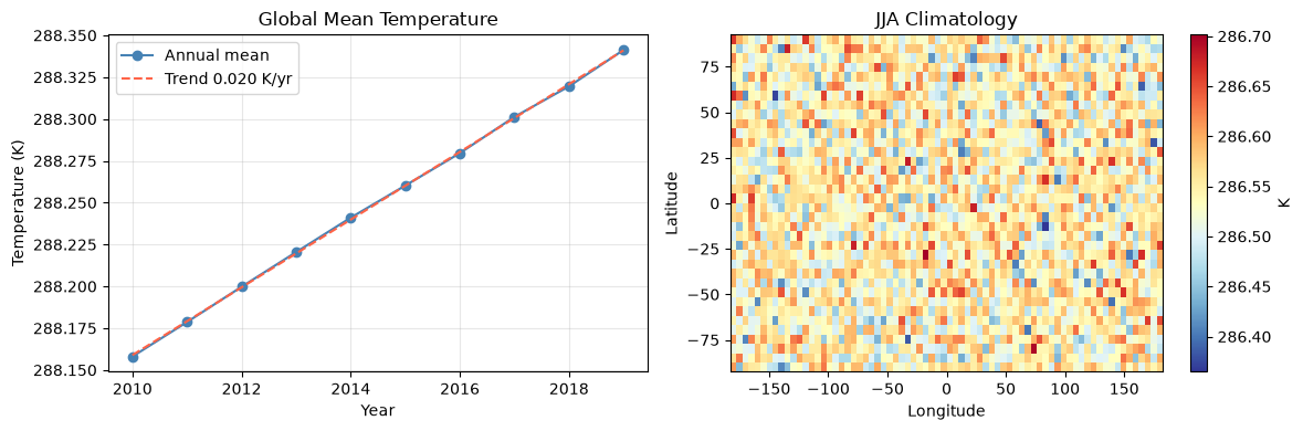
5. Temperature Trend Analysis
Fit a linear trend to the annual global-mean temperature series.
# Global mean temperature time series
global_ts = float(ds_qc.temperature.mean(dim=["lat", "lon"]).mean(dim="time").compute())

# Annual global mean
annual_global = (
    ds_qc.temperature
    .mean(dim=["lat", "lon"])
    .resample(time="1YE")
    .mean()
    .compute()
)

# Linear fit
years = np.arange(len(annual_global))
T_vals = annual_global.values
slope, intercept = np.polyfit(years, T_vals, 1)

print(f"Annual global mean temperature:")
print(f"  First year  : {T_vals[0]:.3f} K")
print(f"  Last year   : {T_vals[-1]:.3f} K")
print(f"  Trend       : {slope:.4f} K/year  ({slope * 10:.3f} K/decade)")
print(f"  Expected    : 0.02 K/year (injected warming rate)")
/opt/hostedtoolcache/Python/3.13.15/x64/lib/python3.13/site-packages/distributed/client.py:3429: UserWarning: Sending large graph of size 36.10 MiB.
This may cause some slowdown.
Consider loading the data with Dask directly
 or using futures or delayed objects to embed the data into the graph without repetition.
See also https://docs.dask.org/en/stable/best-practices.html#load-data-with-dask for more information.
  warnings.warn(
/opt/hostedtoolcache/Python/3.13.15/x64/lib/python3.13/site-packages/distributed/client.py:3429: UserWarning: Sending large graph of size 36.10 MiB.
This may cause some slowdown.
Consider loading the data with Dask directly
 or using futures or delayed objects to embed the data into the graph without repetition.
See also https://docs.dask.org/en/stable/best-practices.html#load-data-with-dask for more information.
  warnings.warn(
Annual global mean temperature:
  First year  : 288.158 K
  Last year   : 288.341 K
  Trend       : 0.0202 K/year  (0.202 K/decade)
  Expected    : 0.02 K/year (injected warming rate)
6. Visualisation
if PLOT:
    fig, axes = plt.subplots(1, 2, figsize=(12, 4))

    # Annual global mean temperature trend
    ax = axes[0]
    ax.plot(years + 2010, T_vals, "o-", color="steelblue", label="Annual mean")
    ax.plot(years + 2010, intercept + slope * years, "--", color="tomato",
            label=f"Trend {slope:.3f} K/yr")
    ax.set_xlabel("Year")
    ax.set_ylabel("Temperature (K)")
    ax.set_title("Global Mean Temperature")
    ax.legend()
    ax.grid(alpha=0.3)

    # Seasonal climatology map (JJA)
    ax = axes[1]
    jja = seasonal_clim.sel(season="JJA")
    im = ax.pcolormesh(LON, LAT, jja.values, cmap="RdYlBu_r", shading="auto")
    plt.colorbar(im, ax=ax, label="K")
    ax.set_xlabel("Longitude")
    ax.set_ylabel("Latitude")
    ax.set_title("JJA Climatology")

    plt.tight_layout()
    fig_path = WORK_DIR / "climate_summary.png"
    plt.savefig(fig_path, dpi=120, bbox_inches="tight")
    print(f"Figure saved to {fig_path}")
    plt.show()
else:
    print("matplotlib not available — skipping plots")
Figure saved to /tmp/climate_case_k8aftkqg/climate_summary.png
7. Save to Zarr
Write the QC’d dataset and derived products to Zarr for fast downstream analysis.
if ZARR:
    # Save QC'd daily data
    qc_store = WORK_DIR / "climate_qc.zarr"
    t0 = time.perf_counter()
    ds_qc.to_zarr(qc_store, mode="w", consolidated=True)
    elapsed = time.perf_counter() - t0

    store_mb = sum(f.stat().st_size for f in qc_store.rglob("*") if f.is_file()) / 1e6
    print(f"QC dataset saved: {qc_store} ({store_mb:.1f} MB, {elapsed:.2f}s)")

    # Verify roundtrip
    ds_check = xr.open_zarr(qc_store, consolidated=True)
    t_check = float(ds_check.temperature.mean().compute())
    print(f"Roundtrip verify — global mean: {t_check:.4f} K")
    ds_check.close()
else:
    print("zarr not available — skipping output")
/opt/hostedtoolcache/Python/3.13.15/x64/lib/python3.13/site-packages/zarr/api/asynchronous.py:246: ZarrUserWarning: Consolidated metadata is currently not part in the Zarr format 3 specification. It may not be supported by other zarr implementations and may change in the future.
  warnings.warn(
/opt/hostedtoolcache/Python/3.13.15/x64/lib/python3.13/site-packages/distributed/client.py:3429: UserWarning: Sending large graph of size 72.19 MiB.
This may cause some slowdown.
Consider loading the data with Dask directly
 or using futures or delayed objects to embed the data into the graph without repetition.
See also https://docs.dask.org/en/stable/best-practices.html#load-data-with-dask for more information.
  warnings.warn(
QC dataset saved: /tmp/climate_case_k8aftkqg/climate_qc.zarr (61.4 MB, 0.42s)
Roundtrip verify — global mean: 288.2499 K
client.close()
cluster.close()

import shutil
shutil.rmtree(WORK_DIR, ignore_errors=True)
print("Cluster closed, temp files removed.")
Cluster closed, temp files removed.
Scaling to Production
To run this workflow at full scale on NCI Gadi:
# In your PBS job script. mode="local" keeps it on the job's node:
# inside a batch job the default mode="auto" picks the multi-node backend.
client, cluster, tmp = setup_dask_client(profile="climate_analysis", mode="local")
# → CPU workload, 60 GB reserve, all the cores PBS gave the job
For very large datasets spanning many nodes, use the v2.0 multi-node API:
from dask_setup import MultiNodeConfig
client, cluster, _ = setup_dask_client(
    mode="pbs",
    multi_node_config=MultiNodeConfig(
        workers_per_node=4, cores_per_worker=12,
        mem_per_worker_gb=32.0, walltime="08:00:00",
    ),
)
See the Multi-Node wiki page for details.