Himawari-AHI cloud type data#
The cloud type product is derived from Himawari AHI data using NWC SAF algorithms included in NWC/GEO software package. The CT product contains information on the major cloud classes: fractional clouds, semitransparent clouds, high, medium and low clouds (including fog) for all the pixels identified as cloudy in a scene.
The dataset derived from the Bureau of Meteorology Satellite Derived Products under various NCI data collection, check the documentation for more details.
This dataset have been post-processed to include the timestamp as a dimension and converted nx/ny to lat/lon coordinates. The domain is the Australian regional domain. Please cite/awknowledge the following people if this data has been used for publications/presentations: Samuel Green - ORCID 0000-0003-1129-4676; Mat Lipson - ORCID 0000-0001-5322-1796; Kimberley Reid - ORCID 0000-0001-5972-6015.
Data location#
/g/data/su28/himawari-ahi
Data format and variables#
The data is available in zarr format, to read it follow the example:
import xarray as xr

ds = xr.open_zarr("/g/data/su28/himawari-ahi/cloud/ct/aus_regional_domain/S_NWC_CT_HIMA08_HIMA-N-NR.zarr/")
ds
Variables:
ct
ct_conditions
ct_cumuliform
ct_multilayer
ct_quality
ct_status_flag
Example code to plot cloud cover#
You can find the example notebook here: g/data/su28/tools/su28_scripts/himawari/himawari_tutorial.ipynb
Or use the code snippet below:
import xarray as xr
import zarr
import re
import matplotlib.pyplot as plt
from matplotlib import colormaps
import matplotlib.colors as mcolors
from matplotlib.colors import LinearSegmentedColormap, TwoSlopeNorm
import matplotlib.cm as cm
import cartopy.crs as ccrs
import cartopy.feature as cft
import cmocean as cmo
import matplotlib as mpl
import matplotlib.ticker as mticker
from dask.distributed import Client
client = Client()
client
ds_z = xr.open_zarr("/g/data/su28/himawari-ahi/cloud/ct/aus_regional_domain/S_NWC_CT_HIMA08_HIMA-N-NR.zarr", consolidated=True)
comment = '1: Cloud-free land; 2: Cloud-free sea; 3: Snow over land; 4: Sea ice; 5: Very low clouds; 6: Low clouds; 7: Mid-level clouds; 8: High opaque clouds; 9: Very high opaque clouds; 10: Fractional clouds; 11: High semitransparent thin clouds; 12: High semitransparent moderately thick clouds; 13: High semitransparent thick clouds; 14: High semitransparent above low or medium clouds; 15: High semitransparent above snow/ice'
# Use regex to extract values and labels
matches = re.findall(r'(\d+):\s+([^;]+)', comment)
# Convert to dictionary
category_dict = {int(num): desc.strip() for num, desc in matches}
# Print result
for k, v in sorted(category_dict.items())[:14]:
print(f"{k}: {v}")
fig = plt.figure(figsize=(16, 8))
ax = plt.axes(projection=ccrs.PlateCarree(central_longitude=130))
ax.coastlines(resolution="50m", color='white')
# Define the values and corresponding colors from tab20
values = [1, 2, 3, 4, 5, 6, 7, 8, 9, 10, 11, 12, 13, 14] # Adjust based on your dataset
# Set the min and max colors from tab20
min_color = mpl.colormaps['tab20'](0 / 20)
max_color = mpl.colormaps['tab20'](19 / 20) # Last color of tab20
# Generate intermediate colors by linearly spacing them within tab20
num_classes = len(values)
colors = [mpl.colormaps['tab20'](i / (num_classes - 1)) for i in range(num_classes)]
# Ensure min/max colors are set explicitly
colors[0] = min_color
colors[-1] = max_color
# Create discrete colormap
cmap = mcolors.ListedColormap(colors)
# Define boundaries for normalization (each value gets its own bin)
boundaries = np.arange(min(values) - 0.5, max(values) + 1.5, 1) # Adjusted for correct binning
norm = mcolors.BoundaryNorm(boundaries, cmap.N)
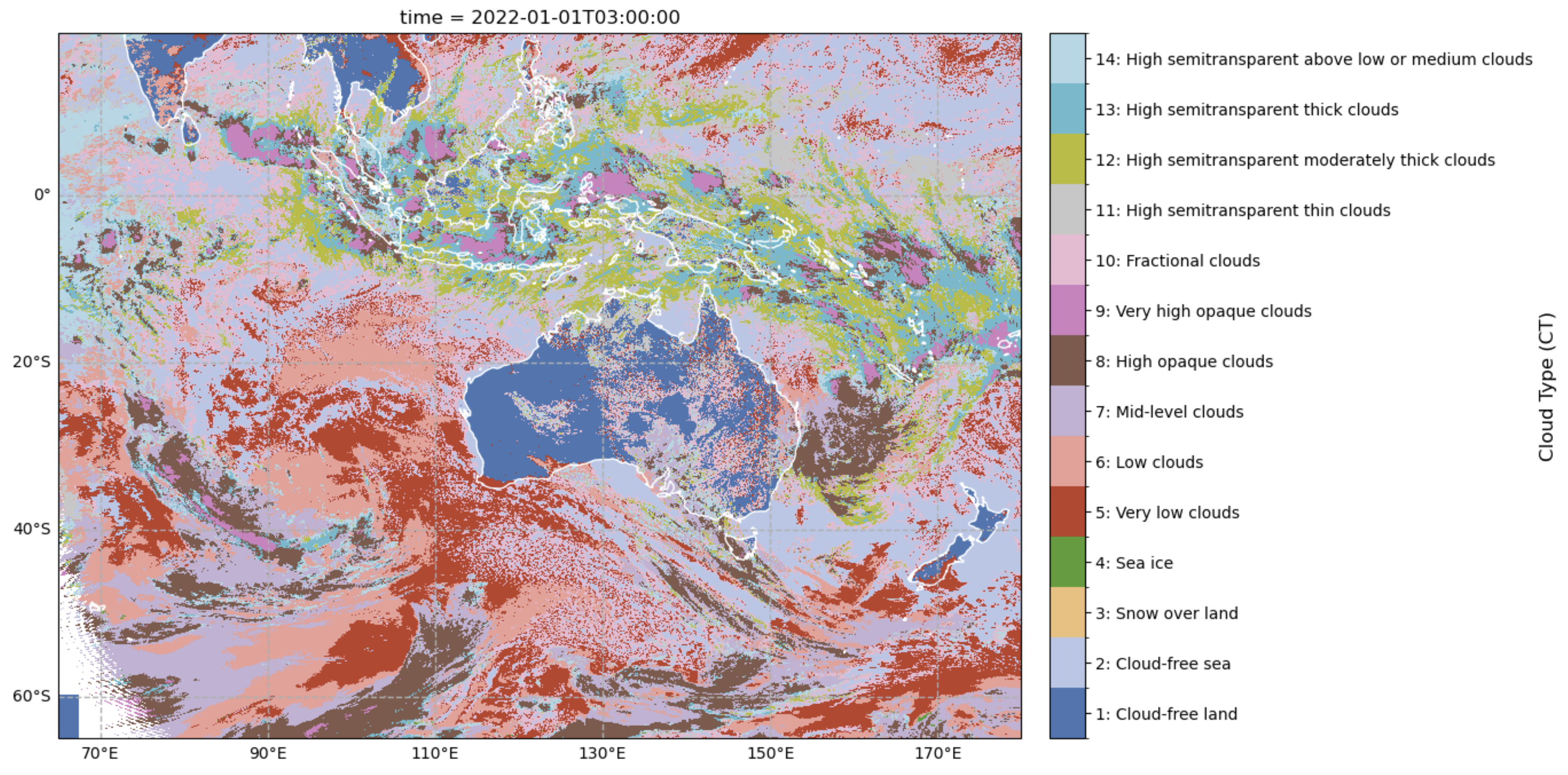
img = ds_z.sel(time='2022-01-01T03:00:00.000000000').ct.plot(ax=ax, x="lon", y="lat", transform=ccrs.PlateCarree(), cmap=cmap, norm=norm, add_colorbar=False)
# Add a discrete colorbar
cbar = fig.colorbar(img, ax=ax, orientation="vertical", fraction=0.03, pad=0.02)
cbar.set_label("Cloud Type (CT)", fontsize=12)
cbar.set_ticks(values) # Ensure ticks match category values
cbar.set_ticklabels([f"{k}: {v}" for k, v in sorted(category_dict.items())[:14]]) # Custom labels
# Add gridlines with labels
gl = ax.gridlines(draw_labels=True, linestyle="--", linewidth=1.0)
gl.top_labels = False # Disable top labels
gl.right_labels = False # Disable right labels
# Increase the number of ticks on the x-axis
gl.xlocator = mticker.FixedLocator(np.arange(70, 190, 20)) # Adjust step size as needed
This gives: