

This is a cross post with the ACCESS-NRI AM3 documentation.
ACCESS-AM3 n512e configuration#
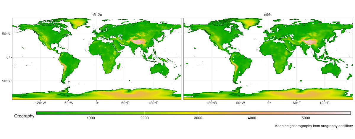
The release-n512e configuration is based on the beta n96e configuration with a few changes to accommodate for the higher resolution requirements. The main changes in the release-n512e configuration are:
Uses climatological aerosols instead of prognostic aerosols.
Modified list of output variables and frequencies (3- and 6-hourly).
The configuration uses a 1024x768 grid, with a nominal resolution of ~25 km and 85 vertical levels.
Initial conditions#
The configuration can be initialise from a n96e or n512e restart. If there is a change of resolution, the reconfiguration step (RECON) will interpolate all the necessary variables.
The suite also include a fix_cable_restart step to populate CABLE variables after the reconfiguration. This is necessary when the model is initialised from low resolution initial conditions.
The default configuration runs with a n96e restart file from January 1, 2007. There may be other restart files available for different dates and resolutions. If you would like to find a restart for your particular purpose, please post in the AM3 subcategory on the Hive Forum.
To change the restart used, edit the file site/nci_gadi.rc:
{% set AINITIAL = '/path/to/restart/file' %}
The initial date and experiment length is defined in the rose-suite.conf_nci_gadi file. The default configuration runs for 1 month, from January 1, 2007.
EXPT_BASIS='20070101T0000Z'
EXPT_RUNLEN='P1M'
Ancilliaries#
The ancillaries n512e where generated using 2 different workflows. The suite u-dj813 was adapted to create the ozone and ESA (sst and sea ice) ancillaries. All the other ancilliaries, including vegetation fraction, vegetation function and soil are generated with the CCI-Ancilliary-Suite and based on the 300m resolution CCI Land Cover dataset.
The following is a summary of the ancilliaries that differ from the beta n96e configuration.
aerosols: monthly mean climatology based on a previous UM run with prognostic aerosols. The climatology is based on the monthly mean of the prognostic aerosols between years 1989 and 2009.veg.fracandand veg.func: based on ESA Land Cover Climate Change Initiative (Land_Cover_cci): Water Bodies Map, v4.0 and Global Land Cover Maps, Version 2.0.7. Centre for Environmental Data Analysis.ozone: monthly mean from 1978 to 2014 based on the CMIP6 dataset: Hegglin, Michaela; Kinnison, Douglas; Lamarque, Jean-Francois; Plummer, David (2016). CCMI ozone in support of CMIP6 - version 1.0. Earth System Grid Federation. https://doi.org/10.22033/ESGF/input4MIPs.1115sstandsea ice: daily mean from 1981 to 2022 based on data from the 0.05° European Space Agency SST Climate Change Initiative (CCI) Analysis v3.0 and associated sea ice concentration data from the EUMETSAT Ocean and Sea Ice Satellite Application Facility (OSI SAF). See https://climate.esa.int/en/projects/sea-surface-temperature/
Output variables#
The variables saved are listed in this spreadsheet. The different groups of variables or “Packages” can be activated/deactivated from the gui.
2D Standard Diagnostics: 2D variables, 3 hourly output
Land Diagnostics: Land variables on tiles, 3 hourly output
3D ERA5 Diagnostics: 37 pressure levels, 6 hourly and monthly mean output
3D Standard Diagnostics: All model levels, 6 hourly and monthly mean output
COSP
2D Extra: extra 2D variables, 3 hourly output
3D Extra: extra 3D variables, 3 hourly output
Currently the COPS, 2D Extra and 3D Extra packages are not active because they haven’t been fully tested. They can be activated from the GUI in
UM/namelist/Model Input and Output/STASH Request and Profiles/STASH request(upper right corner drop-down menu).
Output files are saved in the UM native format in share/data/History_Data/. Some of the variables are saved in monthly files, while others are saved in daily files. Check the spreadsheet to see how the variables are saved.
The output is then converted to netcdf format and saved in share/data/History_Data/netCDF/.
To save space, there is an option to delete the field files after they are converted to netcdf. In app/netcdf_conversion/rose-app.conf, set:
REMOVE_FF=true
Optimization#
The IO Server is active in the configuration to reduce walltime and SU usage. Usually the UM will read and write files on disk sequentially, but the IO Server gets extra processors to read and write files in parallel. This allows the UM to continue with the simulation while the IO Server is writing files to disk.
The current IO Server configuration uses 48 processors divided in 8 tasks, each with 6 workers. This means that it will read/write 8 files in parallel.
The IO Server requires:
rose-suite.congMAIN_IOS_NPROC=48–> number of processors for the IO ServerMAIN_OMPTHR_ATM=2–> number of OpenMP threads
app/um/rose-app.confios_spacing=24–> it’s recommended to spread io processors across the nodesios_tasks_per_server=6–> number of tasks per server.
With a decomposition of 36x36 (MAIN_ATM_PROCX=36, MAIN_ATM_PROCY=36) and the current IO Server configuration, the simulation will use 2688 processors (56 nodes) with a walltime of ~2h 40min per simulated month.